Tame Messy Data: A Step-by-Step Guide to Cleaning Imported Spreadsheets with Power Query
Introduction
If you've ever opened a CSV file only to find jumbled columns, blank rows, misaligned dates, and extra whitespace, you know the frustration of messy imported data. Maybe you inherited a folder full of regional sales reports, or a PDF with shipping costs that needs extraction. The good news: Excel's Power Query (formerly Get & Transform) is a powerful yet often overlooked tool that automates cleaning. This guide walks you through transforming chaotic spreadsheets into a clean, normalized table—step by step. You don't need to be a data analyst; just follow along.
What You Need
- Microsoft Excel (2016 or later, or Office 365) with Power Query enabled (it's built-in)
- A messy imported spreadsheet (CSV, Excel, or text file) to clean
- Basic familiarity with Excel interface (ribbon, menus)
- Patience to apply transformations stepwise
Step 1: Launch Power Query from Your Data Source
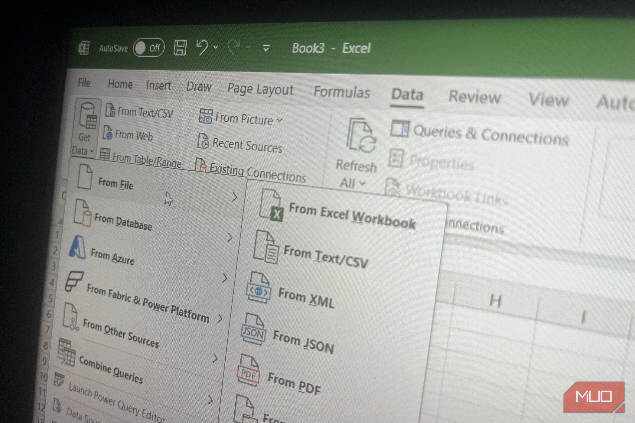
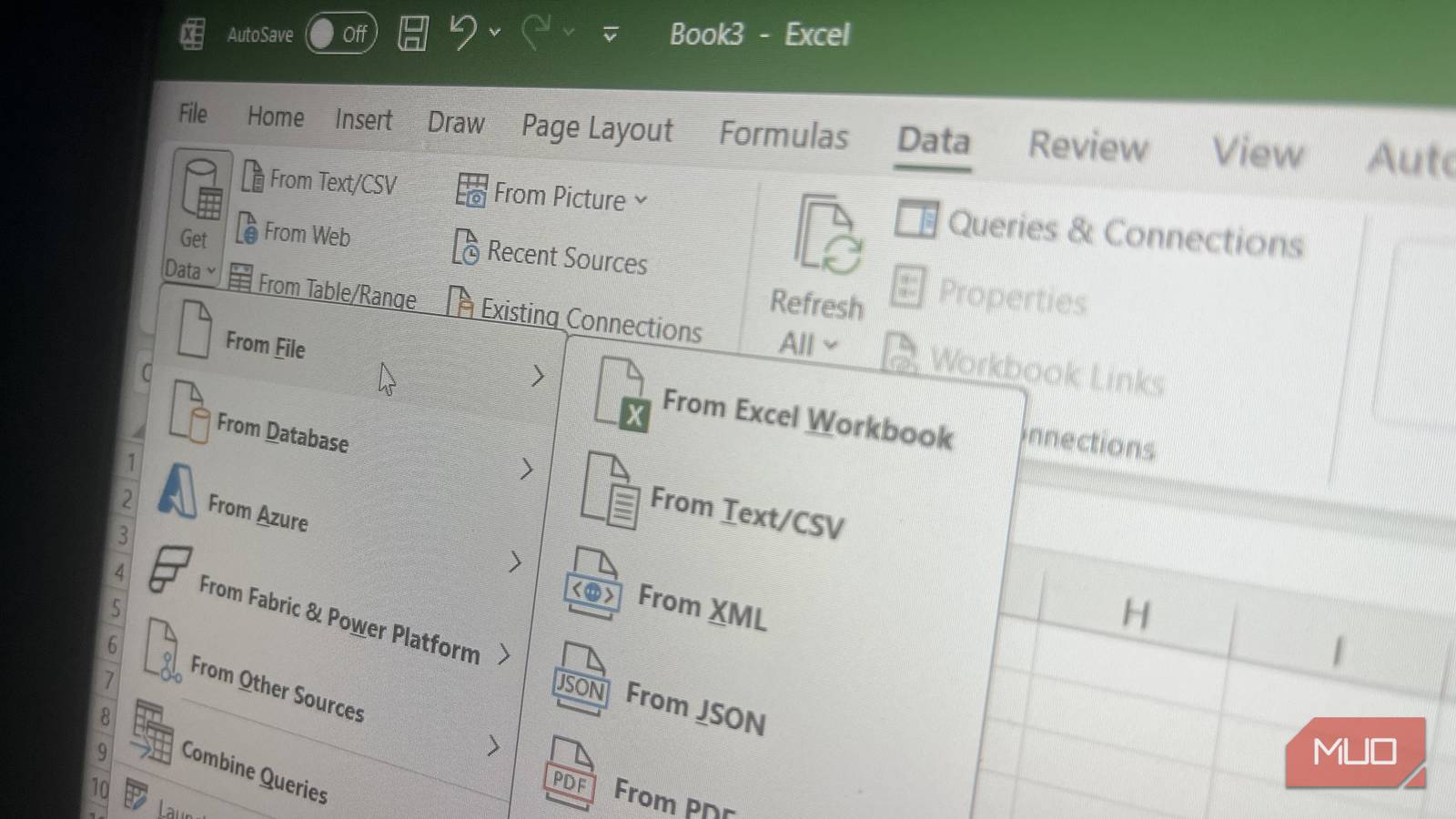
Open Excel and navigate to the Data tab. Click Get Data (or From Text/CSV if you have a CSV). Choose your file. Instead of simply opening it, select Transform Data to launch the Power Query Editor. This opens a dedicated window where you can clean without altering the original file.
Step 2: Promote Headers and Remove Top/Bottom Junk
Look at the preview. Sometimes the first row isn't the header—there might be extra rows with metadata. Use Use First Row as Headers in the Home tab. If there are blank rows or totals at the bottom, remove them: select the rows directly in the preview pane, right-click, and choose Remove Rows. For quick elimination of blank rows, filter the first column for blanks and delete those rows.
Step 3: Change Data Types for Each Column
Power Query auto-detects types (text, number, date), but may guess wrong. Click the icon next to each column header (e.g., ABC for text, # for number, calendar for date) and manually set the correct type. For example, change a column that looks like numbers but has leading zeros to Text to preserve them. This step prevents errors later.
Step 4: Handle Missing or Inconsistent Values
Select a column, go to Transform tab, and use Replace Values to swap nulls, 'N/A', or dashes with blank or 0. To fill downward (common for merged headers), use Fill > Down. For removing duplicates, select the relevant columns, right-click and choose Remove Duplicates. Power Query tracks every action, so you can undo if needed.
Step 5: Split or Merge Columns
Frequently, imported data lumps first and last names, or dates and times, into one column. Select the column, then Split Column > By Delimiter (e.g., space, comma, tab). Alternatively, merge multiple columns by selecting them, right-click, and Merge Columns with a separator. For dates stored as text, use Locale settings in the date type to reformat correctly.
Step 6: Transpose or Unpivot for Normalization
If your data has months across columns instead of rows, you need to unpivot. Select the attribute columns (not the ID columns), then Transform > Unpivot Columns. This creates a tidy three-column table: ID, Attribute, Value. Conversely, use Transpose to swap rows and columns entirely. This step is critical for analyzable formats.
Step 7: Add Index or Custom Columns
To track row order or create a unique key, add an index: Add Column > Index Column. For custom calculations, use Custom Column and write a simple formula (e.g., combine text using &). You can also use conditional columns for groupings. Each new column is applied on the fly.
Step 8: Filter and Sort to Validate
Before loading, apply temporary filters to spot anomalies. Sort by a numeric column to see outliers. Use text filters (contains, starts with) to find data entry errors. Remove rows that fail your validation. Remember: filters in Power Query are permanent once you load, so be sure.
Step 9: Load the Cleaned Data
Once satisfied, click Close & Load from the Home tab. Choose To Table (new worksheet) or To Data Model (for pivot tables). The cleaned data appears in your workbook, and the query is saved. You can refresh later if the source changes by right-clicking the query in the Queries & Connections pane.
Step 10: Save and Document Your Query
Finally, save your Excel file. It's wise to rename the query from 'Query1' to something descriptive (e.g., 'Sales_Cleaned'). Use the Properties pane to add notes. You can also share the file; others can refresh with their own data by updating the source path.
Tips for Success
- Work in the editor: Avoid cleaning manually in the worksheet—Power Query is safer and repeatable.
- Use applied steps: The right pane shows every transformation; click any step to undo or modify.
- Group similar files: Combine multiple CSV files from a folder by using Get Data > From Folder and then Combine & Load.
- Preview before loading: Use data preview filters to check your work.
- Keep the original untouched: Power Query never alters the source file—you can always start over.
- Leverage online resources: Microsoft's Power Query documentation has more complex scenarios like merging queries.
By following these steps, you turn a data mess into a clean, analysis-ready table—all without writing a single macro. Power Query becomes your secret weapon for spreadsheet cleanup.